十天复习CFA一级之数量
- 2026-09-28 02:07:30
使用我学习时的手写的笔记,做成了电子版,然后根据2027年考纲逐条匹配,又用AI编辑了一下格式,适合有一定知识基础、想要自学考CFA一级的人;或者最后一轮复习唤醒记忆的人;或者金融专业的、原计划裸考的人,你总要捋顺一遍考点吧。
实际体验上乐观多了,我复习时用了四天、每天集中精力10小时,就能复习完十科。
CFA一级 · 数量方法
Quantitative Methods · 2027考纲版(不讲原理,只梳理考点)
本讲义按2027年考纲(2027 Level I Topic Outlines)数量科目11个主题、30条LOS编排。
— — — — — — — — — —
使用说明与全局导航
本讲义依据《2027 CFA Level I Topic Outlines》中 Quantitative Methods 科目的学习成果要求(LOS)编制,共 11 个主题、30 条 LOS,适用于已学过一遍教材、考前急速复习的考生,以及金融专业、看一遍即可刷题上考场的学员。Ethics 科目不在此列(网络上有大量优质免费课程)。
Topic 1 · Returns of Financial Assets and Instruments(金融资产与工具的收益)
LOS 1.1 · describe, compare, and interpret returns
Return(收益)是投资在特定持有期内获得的损益,以初始投资价值的百分比表示:
Return = (Ending value − Beginning value + Income) / Beginning value
• Holding period return (HPR):HPR = (P₁ − P₀ + D₁) / P₀,其中 P₀ 为期初价格、P₁ 为期末价格、D₁ 为持有期内收到的收入(股利/利息)。
• Total return vs. price return:总收益包含价格升值(资本利得)与收入两部分;价格收益仅包含价格变动,不含股利/利息收入。
• Real vs. nominal return:(1 + Nominal return)= (1 + Real return) × (1 + Inflation rate)。实际收益剔除了通货膨胀的影响。
• Interpretation & comparison:收益只有在口径一致时才能比较——相同的持有期、相同的币种、风险调整后,并考虑收入与交易成本。
💡 学霸速记 Return 就是投资的“成绩单”。公式记死:Return =(期末价值 − 期初价值 + 期间收入)÷ 期初价值。算 HPR 的时候,分红必须算进分子!只算价格变动那是 Price return(价格收益),算上收入才是 Total return(总收益),这俩不是一回事,考试最爱拿它当干扰项。 |
⚠️ 避坑提醒 名义收益是“面子上”的钱,实际收益是“里子里的钱”。换算用乘法不是加法:(1 + Nominal) = (1 + Real) × (1 + Inflation),千万别直接把名义减通胀当实际——那是近似,考试要的是这个乘法式。收益还要口径一致才能比:同样持有期、同样币种、风险调整后,再算上收入和交易成本。 |
📝 习题演练 An investor purchases a share at $50.00, receives a dividend of $2.00, and sells the share one year later at $53.00. The holding period return is closest to: A. 6.0% B. 10.0% C. 4.0% ✅ 答案:B 📖 解析:HPR = (P₁ − P₀ + D₁)/P₀ = (53 − 50 + 2)/50 = 5/50 = 10.0%。注意必须把股利收入计入分子;若只算价格变动则为6%,选项A是干扰项。 |
LOS 1.2 · describe, compare, and interpret required rates of return, risk-free rates, risk premia, and inflation
• Interest rate is the rate which is charged or paid for the use of money
• Applications of interest rate
• Required rate of return: minimum rate of return an investor must receive in order to accept the investment
• Discounted rate: the rate at which we discount the future amounts to find their value today
• Opportunity cost: the value that investors forgo by choosing a particular course of action
• Nominal interest rate = nominal risk-free interest rate + default risk premium + liquidity premium + maturity premium
• = real risk-free interest rate + inflation rate
利率就是借钱用钱的“代价”,考试老搞混它的三个分身:Required rate of return 是“你最低肯投”的要求回报率,跟相亲底线一个道理;Discount rate 是把未来钱折回今天的“时光折扣率”;Opportunity cost 是你选了 A 放弃 B 的“机会成本”。
⚠️ 避坑提醒 Nominal interest rate = 名义无风险利率 + 违约溢价 + 流动性溢价 + 期限溢价,这“四件套”一个都不能漏!给你 4%、1.5%、0.5%、1.0%,答案就是 7.0%,选 5.5% 的是漏了违约溢价(公司债凭什么比国债高?就高在违约风险上)。还有第二条通道:Nominal = real risk-free rate + inflation rate,两条都要会。 |
📝 习题演练 An analyst observes that the nominal risk-free rate is 4%, the default risk premium is 1.5%, the liquidity premium is 0.5%, and the maturity premium is 1.0%. The nominal interest rate on the risky 5-year corporate bond is closest to: A. 4.0% B. 7.0% C. 5.5% ✅ 答案:B 📖 解析:Nominal interest rate = nominal risk-free interest rate + default risk premium + liquidity premium + maturity premium = 4% + 1.5% + 0.5% + 1.0% = 7.0%。选项C(5.5%)漏掉了default risk premium,是常见错误。 |
Topic 2 · Types of Financial Returns(金融收益的类型)
LOS 2.1 · calculate, compare, and interpret different types of returns for financial assets, instruments, and indicators
• Arithmetic mean return focus on average single-period performance
• Population mean μ = Σ(i=1 to N)Xᵢ / N
• Sample mean X̄ = Σ(i=1 to n)Xᵢ / n
• Advantage: Easy to work with mathematically; Uses all the information about the size and magnitude
• Disadvantage: Sensitive to extreme values
要有权重的概念
• Weighted mean: X̄w = Σ(i=1 to n)wᵢXᵢ = w₁X₁ + w₂X₂ + …… + wₙXₙ
• Weighted mean are mostly used to calculate the portfolio return, or the expected value based on probabilities
• Geometric mean return focus on the profitability of an investment over a multi-period horizon
• G = ⁿ√(X₁X₂X₃…Xₙ) with Xᵢ ≥ 0 for i = 1,2,3,…,n
• Periodic return_compound = ⁿ√(1 + R₁)(1 + R₂)……(1 + Rₙ) − 1
• Harmonic mean: X̄_Harmonic = N / Σ(i=1 to N)(1/Xᵢ)
多只股票,投入资金相等时,求平均 P/E 市盈率,常用调和平均。
调和平均,用来算「固定总量下,平均速率、平均单价」,特点:对小数更敏感。很小的数会大幅拉低调和平均值
看到Dollar-cost averaging闭眼用Harmonic mean
每次投入相同的钱,分批买入,求平均每股成本 → 调和平均
例如:投资者分 2 次,每次投入 $1000(金额相等)买入股票:第 1 次:股价 $10 / 股;第 2 次:股价 $20 / 股 求平均每股购买成本。
验证(实际算股数):第一次 1000 美元:1000/10=100股;第二次 1000 美元:1000/20=50股。总投入 = 2000 美元,总股数 =150 股,平均成本 = 2000/150 =13.33 ✔
❌ 不能用算术平均:(10+20)/2=15,这个是错的!算术平均是每次买相同股数才用。每次投入相同资金 → 调和平均(CFA 必考区分点)
• Comparison among different means: Harmonic Mean ≤ Geometric Mean ≤ Arithmetic Mean
• Equal sign will only be valid given all the observations are same
• Greater variability of the different observation, the more the arithmetic mean will exceed the geometric mean and harmonic mean as well
💡 学霸速记 均值家族开会,外号记牢:算术平均是“直线脑”,管单期平均表现,好用但会被极端值带偏;几何平均是“复利脑”,管多期复利,才是投资“真话”版,算收益率要先把每个 1+R 乘起来再开 n 次根再减 1;调和平均是“平均速度脑”,专门用来算定投的平均成本(每次投同样钱、买不同价格)。 |
⚠️ 避坑提醒 经典送分题:第一年 +20%、第二年 −20%,算术平均 0% 看着没亏,其实你的 100 块先变 120 再跌回 96,真亏了 4%!几何平均 ≈ −2.02% 才是真相。所以题目问“长期盈利能力”、给你多期收益率 → 必选几何平均;问“单期平均表现”才用算术。还有个不等式:Harmonic ≤ Geometric ≤ Arithmetic,波动越大算术越虚高。持有 6 个月赚 5%,年化别用 5%×2,要按复利 (1.05)²−1≈10.25%,考试认复利版。 |
📝 习题演练 A portfolio earns +20% in Year 1 and −20% in Year 2. Compared with the arithmetic mean return, the geometric mean return over the two years is most likely: A. higher B. lower C. equal ✅ 答案:B 📖 解析:算术平均 = (20% − 20%)/2 = 0%;几何平均 = √(1.20 × 0.80) − 1 = √0.96 − 1 ≈ −2.02% < 0%。观测值波动越大,算术平均越超过几何平均(Harmonic ≤ Geometric ≤ Arithmetic)。几何平均正确反映了复利效应。 |
Topic 3 · Benchmarking Returns(收益基准(衡量与指数))
LOS 3.1 · calculate and compare money-weighted and time-weighted rates of return
• Time-weighted rate of return (TWRR):以各子期间的几何平均(链式复合)衡量组合表现,剔除资金流入/流出的影响。TWRR = (1 + r₁)(1 + r₂)…(1 + rₙ) − 1,其中 rₜ 为各子期间的收益率。
• Money-weighted rate of return (MWRR):即投资现金流的内部收益率 IRR(令 PV(流入) = PV(流出) 的折现率),受投资者追加/撤回资金的时点与金额影响。
• 比较与使用:评价组合经理业绩用 TWRR(经理不控制现金流时最公平);评价投资者实际获得的收益用 MWRR。资金投入集中在表现好(差)的期间时,MWRR 高于(低于)TWRR。
💡 学霸速记 记住两条:TWRR 是“经理的成绩单”,MWRR 是“你自己的钱包”。TWRR 把各子期间收益链式复合((1+r₁)(1+r₂)…−1),剔除了客户啥时候加钱、取钱的影响;MWRR 就是现金流的 IRR,钱什么时候进、什么时候出都直接影响结果。 |
⚠️ 避坑提醒 题目问 “evaluating the performance of the portfolio manager”,闭眼选 Time-weighted rate of return——经理管不了客户啥时候打钱,别用 IRR 冤枉他。资金投入集中在表现好的期间,MWRR 会高于 TWRR;反之则低。 |
📝 习题演练 An investor contributes $100,000 just before a period in which the portfolio returns +20%, then withdraws $50,000 just before a period in which the portfolio returns −10%. Which measure is most appropriate for evaluating the performance of the portfolio manager? A. The money-weighted rate of return B. The time-weighted rate of return C. The holding period return ✅ 答案:B 📖 解析:TWRR 通过链式复合各子期间收益,剔除了投资者资金进出时点与规模的影响,因此是评价组合经理(不控制现金流)业绩的标准指标。MWRR(IRR)会因资金流进出而扭曲经理的真实表现。 |
LOS 3.2 · describe the choices and the implications of the different weighting methods used in index construction and management, and calculate, interpret, and explain the value and the returns of an index
说是describe,只要知道他们各自的特点,能选出正确选项即可。等二级时考计算,也是在想象出他们各自的特点的基础上,再想象一下为啥有这个特点?→计算方法导致的它有这个特点→计算方法是xxx,这样就能计算了。等三级时不会让你写essay去describe的。
• Price-weighted index(价格加权):Index value = Σ股票价格 / Divisor。高价股影响大;发生拆股(stock split)时必须调整除数,否则指数会失真。典型:道琼斯工业平均指数。
• Equal-weighted index(等权加权):对每只成分股的收益率取简单平均(定期再平衡)。小市值股被给予与大盘股同等的权重,波动通常更大。
• Market-capitalization-weighted index(市值加权,也称价值加权):权重 = 个股市值 / 总市值 = (Pᵢ×Qᵢ)/Σ(Pⱼ×Qⱼ)。大盘股主导指数表现,无需因拆股调整,无需再平衡。典型:标普500、沪深300。
• Float-adjusted market-cap weighting(自由流通市值加权):只按可自由流通的股份计算市值,剔除控股股东等非流通股份。
• 指数价值与收益:Index value 反映加权组合的价值;Index return = (Index value₁ − Index value₀)/Index value₀(含再投资口径可得总收益指数)。
💡 学霸速记 三种加权记外号:价格加权是“大佬说了算”(股价越高权重越大,典型道琼斯);等权是“人人平等”(每只股票收益率简单平均,小票大票同权,波动大);市值加权是“按钱排座次”(权重=个股市值/总市值,大盘股主导,典型标普500、沪深300)。 |
⚠️ 避坑提醒 哪个指数最怕拆股?价格加权!一只票 1 拆 2,价格腰斩,指数就得调除数(divisor)补救;市值加权是“价格×股数”,拆股后市值不变,完全无感;等权按收益率平均,跟绝对价格也没关系。看到 stock split → 锁定价格加权;看到 large-cap dominates / no rebalancing → 锁定市值加权。 |
📝 习题演练 Which index weighting method is most likely to be affected by a stock split in one of its constituent securities? A. A price-weighted index B. A market-capitalization-weighted index C. An equal-weighted index ✅ 答案:A 📖 解析:价格加权指数将成分股价格加总并除以除数;拆股直接改变个股价格,若不调整除数将扭曲指数。市值加权指数以“价格×股数”计算权重,拆股不影响总市值;等权指数按收益率平均,也与绝对价格无关。 |
Topic 4 · The Time Value of Money in Finance(货币时间价值)
LOS 4.1 · calculate and interpret the present value of fixed-income and equity instruments based on expected future cash flows
• Present value (PV) is the value of an initial investment
• Future value (FV) is the value of an initial investment would be worth in the future
• Compounding: FV = PV × (1 + r)ⁿ
• Discount: PV = FV / (1 + r)ⁿ
• r is the periodic rate, n is the number of periods
• Annuity is a set of constant sequential cash flows
• Ordinary annuity: all constant cash flows occurring at the end of each period
• Annuity due: all constant cash flows occurring at the beginning of each period
• Perpetuity: a set of constant never-ending sequential cash flows occurring at the end of each period
• Present value of perpetuity = perpetuity annuity / r
• 固定收益(债券):PV = Σ CFₜ/(1+r)ᵗ = C/(1+r) + C/(1+r)² + … + (C + FV)/(1+r)ⁿ,这个一定要会按计算器!在B站找任意一家机构的免费视频。其中 C 为每期票息、FV 为面值、r 为要求的到期收益率(YTM)、n 为期数。
• 权益(股利贴现):零增长模型 PV = D/r;戈登增长模型 PV = D₁/(r − g),其中 D₁ 为下一期股利、r 为要求回报率、g 为股利增长率(须 r > g)。
⚠️ 避坑提醒 债券定价就是把每期票息和到期面值全部折现加总。关键记住:票息率(coupon rate)和到期收益率(YTM)不是一回事!票息率决定每期收多少现金,YTM 是要求回报率。比较时永远拿 coupon rate 和 YTM 比:票息率 |
📝 习题演练 A 3-year bond pays an annual coupon of 5% on a par value of $100 and is priced to yield 6% (annual compounding). The bond's present value is closest to: A. $97.33 B. $100.00 C. $94.00 ✅ 答案:A 📖 解析:PV = 5/1.06 + 5/1.06² + 105/1.06³ = 4.717 + 4.450 + 88.160 ≈ $97.33。票息率(5%)低于收益率(6%),债券折价交易,故价格低于面值100;选项B是票息率=收益率的情形。 |
LOS 4.2 · calculate and interpret the implied return of fixed-income instruments and required return and implied growth of equity instruments given their present value and cash flows
由价格与现金流反解收益率:只要记住上边的公式,下边这个自然而然就能自己推导了。但一级考的更多的还是CAPM模型来计算股票收益率。
• 固定收益——到期收益率(YTM):给定价格 PV 与各期现金流,使 PV = Σ CFₜ/(1+y)ᵗ 成立的折现率 y 即 YTM,是债券的内部收益率。
• 权益——要求回报率:由戈登模型变形 r = D₁/P₀ + g(股利收益率 + 股利增长率)。
• 权益——隐含增长率:给定价格与现金流,g = r − D₁/P₀。
反过来也要会:知道价格反推收益率。债券的 YTM 就是让 PV=ΣCFₜ/(1+y)ᵗ 成立的 y,本质是债券的 IRR。股票由戈登模型变形:要求回报率 r = D₁/P₀ + g(股利收益率 + 增长率)。
⚠️ 避坑提醒 算隐含增长率就用 g = r − D₁/P₀。例:40 块的股票明年股利 2 块,r=10%,g = 10% − 2/40 = 10% − 5% = 5%。别把股利收益率加回去(那是 15%,方向反了)。 |
📝 习题演练 A stock is currently priced at $40.00 and is expected to pay a dividend of $2.00 next year. If the required rate of return is 10%, the implied long-run dividend growth rate is closest to: A. 5.0% B. 15.0% C. 8.0% ✅ 答案:A 📖 解析:由 P₀ = D₁/(r − g) 得 g = r − D₁/P₀ = 10% − 2/40 = 10% − 5% = 5.0%。选项B(15%)是把股利收益率加回了要求回报率,方向错误。 |
LOS 4.3 · explain the cash flow additivity principle and its importance for the condition of no arbitrage, and explain its use in calculating implied forward interest rates, forward exchange rates, and option values
• Cash flow additivity(现金流可加性):一组现金流的现值等于各现金流现值之和,即 PV(CF₁ + CF₂) = PV(CF₁) + PV(CF₂)。它是“无套利(no arbitrage)”定价的基础:若两个组合未来现金流完全相同,其价格必须相同,否则存在套利机会。
• 隐含远期利率(implied forward rate):由即期利率曲线推出。1年后再投1年的远期利率:f = (1+s₂)²/(1+s₁) − 1,其中 s₁、s₂ 分别为1年期、2年期即期利率。
• 远期汇率(forward exchange rate):由利率平价(covered interest rate parity)推出:F = S × (1+r_d)/(1+r_f),其中 S 为即期汇率、r_d 为本币利率、r_f 为外币利率。
• 期权价值:期权可视为未来现金流的组合(复制组合),其价值亦由“无套利+现金流复制”得出(如无风险组合/风险中性定价),此处仅要求理解可加性与无套利的作用。
💡 学霸速记 现金流可加性一句话:一组现金流的现值 = 各现金流现值之和。它是无套利定价的地基——两个组合未来现金流完全一样,价格就必须一样,不然就套利薅羊毛。 |
⚠️ 避坑提醒 隐含远期利率不是两个即期利率的平均!(3%+4%)/2 这种平均法是 100% 错的。远期利率是“未来那一年的边际借款成本”,必须用 f=(1+s₂)²/(1+s₁)−1 算。例:s₁=3%、s₂=4% → f=1.04²/1.03−1≈5.01%。 |
📝 习题演练 The one-year spot rate is 3.0% and the two-year spot rate is 4.0% (annual compounding). The implied one-year forward rate one year from today is closest to: A. 5.0% B. 4.0% C. 3.5% ✅ 答案:A 📖 解析:f = (1+s₂)²/(1+s₁) − 1 = 1.04²/1.03 − 1 = 1.0816/1.03 − 1 ≈ 5.01%。若套用两个即期利率直接平均(4%)则错误;远期利率反映的是“未来一年”的边际借款成本。 |
Topic 5 · Statistical Characteristics of Asset Returns(资产收益的统计特征)
LOS 5.1 · calculate, interpret, and evaluate various measures of (1) central tendency and location and (2) dispersion
• Population mean μ = Σ(i=1 to N)Xᵢ / N;Sample mean X̄ = Σ(i=1 to n)Xᵢ / n
• Weighted mean: X̄w = w₁X₁ + w₂X₂ + …… + wₙXₙ;mostly used to calculate the portfolio return, or the expected value based on probabilities
• Geometric mean: G = ⁿ√(X₁X₂X₃…Xₙ);Harmonic mean: X̄_Harmonic = N / Σ(1/Xᵢ);Harmonic Mean ≤ Geometric Mean ≤ Arithmetic Mean
• Median is the value of the middle item of a set of ascending or descending order
• Odd number of n items, median occupies the (n+1)/2 position; Even number of n items, median is equal to the mean of the items occupying the n/2 and (n+2)/2 positions
• Median Advantage: not affected by extreme values (a.k.a., outliers) as arithmetic mean; Disadvantage: only one or two numbers considered, rest is to be ignored
• Mode is the most frequently occurring value of the distribution; The distribution could have more than one mode, or even no mode
• Quantile is a value at or below which a stated fraction of the data lies
• Quartiles: quarters; Quintiles: fifths; Deciles: tenths; Percentiles: hundredths
• Formula for location of data in ascending order: Lᵧ = (n+1)y/100(y is the yᵗʰ percentile, n is the number of data)
• Example: For data with 17 observations, location of 3ʳᵈ quintile: Lᵧ = (17+1)×0.60 = 10.8, i.e., eight-tenths of the way from the 10ᵗʰ to the 11ᵗʰ observation
• Dispersion describes the variability around the central tendency, usually used to address the risk
• Range = maximum value – minimum value(Easy for computation, but only use two numbers and tell nothing about the distribution of the data set)
• MAD = Σ(i=1 to n)|Xᵢ − X̄| / n
• Population variance σ² = Σ(i=1 to N)(Xᵢ − μ)² / N;Sample variance s² = Σ(i=1 to n)(Xᵢ − X̄)² / (n−1)
• Population standard deviation σ = √σ²;Sample standard deviation s = √s²
💡 学霸速记 中位数外号“排队中间那位”:排好序,奇数个取中间那个(位置 (n+1)/2),偶数个取中间两个的平均。它的优点是抗极端值——一个亿万富翁进小区,平均收入瞬间上天,中位数纹丝不动。众数“人气王”,出现次数最多,可以有好几个也可以一个都没有。分位数“排队切段”:四分位、五分位、十分位、百分位。 |
⚠️ 避坑提醒 分位数位置公式是 Lᵧ=(n+1)y/100,括号里是 (n+1) 不是 n!多少人把 25 代进去算成 18.75,全错。这个 +1 是 CFA 最爱埋的雷。另外离散程度看“飘不飘”:算样本方差分母必须是 n−1(样本均值是自己算的,自由度少了一个),不是 N,这也是高频坑。 |
📝 习题演练 An analyst has ranked 25 observations in ascending order. The location of the third quartile in the ordered data is closest to: A. the 18.5th position B. the 19.5th position C. the 20.5th position ✅ 答案:B 📖 解析:Lᵧ = (n+1)y/100 = (25+1)×75/100 = 19.5,即第三四分位数位于第19个与第20个观测值之间的中点。选项A(18.5)是把(n)代入而忘了+1;选项C是第五分位数口径。 |
LOS 5.2 · describe, interpret, and evaluate measures of skewness and kurtosis
• Skewness indicates the degree of symmetry of return distributions
• 1. Sₖ = 0, symmetrical distribution, Mean = Median = Mode
• 2. Sₖ > 0, positively (right) skewed distribution, Mode < Median < Mean
• 3. Sₖ < 0, negatively (left) skewed distribution, Mean < Median < Mode
• Kurtosis measures the degree to which the distribution is more or less peaked than normal distribution
• Excess kurtosis = kurtosis − 3
• 1. Leptokurtic: Fatter tailed than normal distribution; Kurtosis > 3, excess kurtosis > 0
• 2. Mesokurtic: Identical to normal distribution; Kurtosis = 3, excess kurtosis = 0
• 3. Platykurtic: Thinner tailed than normal distribution; Kurtosis < 3, excess kurtosis < 0
标准正态分布的偏度(skewness)= 0,峰度(kurtosis)= 3,Excess Kurtosis,即 “相对标准正态多出来的部分”= 0
💡 学霸速记 形状三兄弟看“尾巴”:偏度看尾巴朝哪边——正偏(右偏)长尾在右,Mode <Median<Mean,均值被右侧极端大值拉走(像彩票,大部分人亏、少数人暴富);负偏(左偏)反之,Mean<Median </Median<Mean,均值被右侧极端大值拉走(像彩票,大部分人亏、少数人暴富);负偏(左偏)反之,Mean<Median |
⚠️ 避坑提醒 峰度看“尖胖扁瘦”:Leptokurtic 尖峰厚尾(kurtosis>3,excess>0)、Mesokurtic 正态(=3,excess=0)、Platykurtic 平峰薄尾(<3,excess<0)。金融资产收益最爱“尖峰厚尾”——极端暴跌比正态预测的更多,这就是为什么 2008 没人算得到。 |
📝 习题演练 A distribution of returns is described by Mode < Median < Mean. Which statement is most accurate? A. The distribution is negatively skewed B. The distribution is positively (right) skewed and the mean is pulled toward the right tail C. The distribution is symmetric about its mean ✅ 答案:B 📖 解析:偏度系数 Sₖ > 0 时为正偏(右偏):Mode < Median < Mean,长尾在右侧,均值被极端大值拉向右尾。负偏则反之(Mean < Median < Mode)。 |
LOS 5.3 · calculate, interpret, and evaluate covariance and correlation
• Covariance is a measure of how two pair variables move together
• Cov(X,Y) = E {[X − E(X)]×[Y − E(Y)]};Covariance measures the linear relationship between two variables
• 1. Positive covariance: Two variables tend to be above or below their expected values at the same time; tend to increase or decrease at the same time
• 2. Negative covariance: One variable tend to be above its expected value when the other is below its expected value; tend to increase when the other decreases
• 3. Zero covariance: no linear relationship between two variables
• Autocovariance is equal to the variance; Covariance values range from negative infinity to positive infinity
• Correlation is a standardized measure of linear relationship between two variables
• ρᵢ,ⱼ = Cov(Rᵢ,Rⱼ)/σᵢσⱼ(总体);rᵢ,ⱼ = Cov(Rᵢ,Rⱼ)/sᵢsⱼ(样本)
• Correlation values range from +1 (perfect positive correlation) to −1 (perfect negative correlation)
• Example: E(X)=13, E(Y)=18; COV(X,Y)=15%(20−13)(40−18)+60%(15−13)(20−18)+25%(4−13)(0−18)=66
💡 学霸速记 协方差和相关系数是:协方差正→同涨同跌,负→你涨我跌,零→没关系。但协方差大小没法跨组比较,所以标准化成相关系数 ρ=Cov/(σᵢσⱼ),范围 [−1,+1]。 |
⚠️ 避坑提醒 算相关系数:ρ = Cov / (σA×σB)。例:协方差 0.024,σA=0.40,σB=0.30 → ρ = 0.024/(0.40×0.30) = 0.20。把协方差除以两个标准差,就得到没单位、可跨资产比的系数。 |
📝 习题演练 The covariance between the returns of two assets is 0.0240. Asset A has a standard deviation of 0.40 and Asset B has a standard deviation of 0.30. The correlation between the two assets is closest to: A. 0.20 B. 0.32 C. 0.03 ✅ 答案:A 📖 解析:ρ = Cov(R_A,R_B)/(σ_A×σ_B) = 0.0240/(0.40×0.30) = 0.0240/0.12 = 0.20。相关系数把协方差标准化到[−1,+1]区间,可直接跨资产比较。 |
LOS 5.4 · calculate, interpret, and evaluate semi-deviation and coefficient of variation
• The target downside deviation (a.k.a. target semi-deviation) is a measure of dispersion of the below the target
• Sample target semi-deviation formula: s_Target = √[Σ(for all Xᵢ ≤ B)(Xᵢ − B)² / (n − 1)]
• B is the target; n is the total number of sample observations
• Coefficient of variation (CV) is a measure of risk per unit of mean return, thus the lower is better
• CV = s / x̄
• CV has no units of measurement, so permits direct comparisons of dispersions across different data sets
💡 学霸速记 下行偏差只管“低于目标”那部分波动——涨得猛不是风险,跌得狠才是。变异系数 CV = s/x̄,外号“每单位收益背多少风险”,越低越好,而且无量纲,跨基金随便比。 |
⚠️ 避坑提醒 看到 “lower is better / no units” → 锁定 CV;看到 “below the target” → 锁定 semi-deviation。例:基金 X 均值 12%、标准差 18% → CV=1.5;基金 Y 均值 8%、标准差 14% → CV=1.75。CV 越小越好,X 赢。 |
📝 习题演练 Fund X has a mean return of 12% and a standard deviation of 18%; Fund Y has a mean return of 8% and a standard deviation of 14%. Based on the coefficient of variation, which fund provides more return per unit of risk? A. Fund X B. Fund Y C. The two funds are identical ✅ 答案:A 📖 解析:CV_X = 18/12 = 1.50;CV_Y = 14/8 = 1.75。CV越低说明单位收益承担的风险越小,故Fund X更优。注意CV无量纲,可直接跨不同均值水平的数据集比较。 |
Topic 6 · Statistical Distributions for Financial Asset Prices and Returns(金融资产价格与收益的统计分布)
LOS 6.1 · calculate, interpret, and evaluate unconditional expected values for mean, variance, and covariance
• Expected value is the probability weighted average of the possible outcomes of the random variable X
• E(X) = P(X=x₁)×x₁ + P(X=x₂)×x₂ + …… + P(X=xₙ)×xₙ
• Variance: σ²(X) = P(X=x₁)×[x₁ − E(X)]² + P(X=x₂)×[x₂ − E(X)]² + …… + P(X=xₙ)×[xₙ − E(X)]²
• Standard deviation: Positive squared root of variance
• Example: Recession 25% → −0.10; Normal 50% → 0.08; Boom 25% → 0.22; E(X) = 0.07, σ² = 0.01290
• Cov(X,Y) = E {[X − E(X)]×[Y − E(Y)]};Autocovariance is equal to the variance
💡 学霸速记 期望值就是“概率加权平均”,不是简单平均!E(X)=Σ P(X=xᵢ)×xᵢ。方差是每个取值到期望的平方、再按概率加权:σ²(X)=Σ P(xᵢ)×[xᵢ−E(X)]²。算期望要把每种情况的收益乘上它发生的概率再全部相加。 |
📝 习题演练 An analyst estimates the following return distribution for an asset: Probability 20% → return 12%; Probability 50% → return 8%; Probability 30% → return −4%. The expected return is closest to: A. 5.2% B. 8.0% C. 5.0% ✅ 答案:A 📖 解析:E(X) = 0.20×12% + 0.50×8% + 0.30×(−4%) = 2.4% + 4.0% − 1.2% = 5.2%。期望值是概率加权平均,不是简单平均(选项B为最大概率状态值,选项C为简单平均8/3≈2.67%的误算干扰)。 |
LOS 6.2 · calculate, interpret, and evaluate the principal moments of key statistical distributions used in finance
• Discrete random variable: takes on a countable number of possible values; Continuous random variable: takes on an uncountable number of possible values
• Probability function specifies the probability that the discrete random variable takes on a specific value: P(X = xᵢ)
• Probability density function (PDF) specifies the probability that the continuous random variable takes on a value within a range; the area under the curve indicates the interval; P(x₁ < X < x₂) = ∫ₓ₁ˣ² f(x)dx, P(X = xᵢ) = 0
• Cumulative probability function (CDF): F(xᵢ) = P(X ≤ xᵢ); P(x₁ < X ≤ x₂) = F(x₂) − F(x₁)
• Discrete uniform distribution has a finite number of possible outcomes, all of which are equally likely
• Binomial random variable (X) represents the number of successes in n Bernoulli trials, assuming that: The probability of success (p) is constant for all trials; The trials are all independent; X ~ B(n, p)
• Expected value for binomial random variable = n×p; Variance = n×p×(1−p)
• P(X = x) = Cₙˣ × pˣ × (1−p)ⁿ⁻ˣ
• Normal distribution: X ~ N(μ, σ²); Completely described by mean and variance; Skewness = 0; Kurtosis = 3; Linear combination of normally distributed random variables is also normally distributed; tails go on forever
• 68% CI = μ ± 1σ; 90% CI = μ ± 1.65σ; 95% CI = μ ± 1.96σ; 99% CI = μ ± 2.58σ
• Standard normal distribution (Z-distribution): μ = 0, σ = 1; Standardization: z = (X − μ)/σ; Φ(−x) = 1 − Φ(x)
• Lognormal: If X is normally distributed, then eˣ is lognormal distributed; bounded from below by zero; positively skewed; can be used to model asset prices
• Continuous uniform distribution: f(x) = 1/(b−a) for a < x < b, 0 otherwise
• Student's T-distribution: defined by single parameter df = n − 1; Symmetrical (bell shaped), skewness = 0; Fatter tails than a normal distribution; As df increase, t-distribution is approaching to standard normal distribution; Given a degree of confidence, t-distribution has a wider confidence interval than z-distribution
卡方分布(Chi-square)与F分布(2027考纲要求“key statistical distributions used in finance”):
• Chi-square (χ²) distribution:k个标准正态随机变量的平方和,即 χ² = ΣZᵢ²,服从自由度 k 的χ²分布;仅取非负值、右偏;随自由度增大趋近正态。E(χ²) = k, Var(χ²) = 2k。用于方差检验。
• F distribution:两个独立χ²变量分别除以其自由度后的比值,F = (χ²₁/df₁)/(χ²₂/df₂);右偏、仅取非负;用于两个总体方差的比较(如F = S₁²/S₂²)及回归的整体显著性检验。
💡 学霸速记 先分清变量:离散随机变量“能数出来”(抛硬币正面几次),连续随机变量“无限多取值”(收益 3.14159…%)。连续变量单点概率 P(X=x)=0,概率只能按区间算(曲线下面积),CDF 是累积到某点的概率 F(x)=P(X≤x)。二项分布外号“抛硬币的数学化”:n 次独立试验、成功概率 p 不变,期望=np、方差=np(1−p)。正态分布“钟形罩”是绝对主角,只用均值和方差就能完全描述,置信区间口诀必背:68% 在 μ±1σ,90% 在 μ±1.65σ,95% 在 μ±1.96σ,99% 在 μ±2.58σ。 |
⚠️ 避坑提醒 对数正态外号“下限为 0 的偏科生”:X 正态则 eˣ 对数正态,下限 0、右偏,正好模拟资产价格(价格不可能为负)。T 分布“胖尾巴小样本”:参数 df=n−1,尾巴比正态肥,df 越大越接近标准正态,同样置信水平下 t 的区间比 z 宽,样本小、方差未知就用 t。2027 新补:方差检验用卡方 χ²、两个方差比较用 F。记死:正态用 z、小样本方差未知用 t、方差检验用 χ²、两方差比用 F。二项算概率要看清试验次数 n,题目常拿 n=5 的答案来坑你。 |
📝 习题演练 The daily probability that a stock rises is 60%. Assuming independent trading days, the probability that the stock rises on exactly 3 of the next 6 trading days is closest to: A. 27.65% B. 34.56% C. 18.66% ✅ 答案:A 📖 解析:P(X=3) = C₆³ × 0.6³ × 0.4³ = 20 × 0.216 × 0.064 = 0.27648 ≈ 27.65%。选项B(34.56%)对应5天中恰好3天上涨(n=5的情形),注意区分试验次数n。 |
LOS 6.3 · calculate, interpret, and evaluate conditional expectations, variances, and covariances
• Unconditional probability (marginal probability): Probability of an event A is not conditioned on another event, denoted P(A)
• Conditional probability: Probability of an event A is conditioned on another event B, denoted P(A|B)
• For independent events: P(A|B) = P(A)
• Joint probability is the probability of event A and B both happen, denoted P(AB)
• P(A|B) = P(AB) / P(B); P(AB) = P(B)×P(A|B) = P(A)×P(B|A)
• Probability that at least one of two events occur, denoted as P(A+B): P(A + B) = P(A) + P(B) − P(AB)
条件期望、条件方差与条件协方差(2027考纲新增的计算与评价要求,讲义只讲了条件概率):
• Conditional expectation:给定另一个随机变量取值条件下的期望,记为 E(X | Y = y);无条件期望可由条件期望加权求得:E(X) = Σᵢ E(X | Sᵢ) × P(Sᵢ)(全期望公式,Total Probability Rule for Expectations)。
• Conditional variance:Var(X | Y = y) = E[(X − E(X|Y=y))² | Y = y],衡量给定Y=y时X围绕其条件期望的离散程度。
• Conditional covariance:Cov(X, Z | Y = y) = E[(X − E(X|Y=y))(Z − E(Z|Y=y)) | Y = y],衡量给定Y条件下X与Z的线性联动。
• 注意:条件期望是Y的函数;无条件期望对条件期望再取期望即可(迭代期望法则)。
💡 学霸速记 条件期望就是“给定某个状态下的期望”。无条件期望用全期望公式把条件期望按状态概率加权:E(X)=Σᵢ E(X|Sᵢ)×P(Sᵢ)。 |
⚠️ 避坑提醒 例:状态1概率 60%、条件期望 10;状态2概率 40%、条件期望 4 → E(X)=10×0.6+4×0.4=6+1.6=7.6。别只取最大的那个,也别简单平均——要乘上状态概率再相加。 |
📝 习题演练 An analyst estimates E(X | State 1) = 10 with P(State 1) = 60%, and E(X | State 2) = 4 with P(State 2) = 40%. The unconditional expected value E(X) is closest to: A. 7.6 B. 7.0 C. 6.4 ✅ 答案:A 📖 解析:E(X) = E(X|S₁)×P(S₁) + E(X|S₂)×P(S₂) = 10×0.60 + 4×0.40 = 6.0 + 1.6 = 7.6。这是全概率法则在期望上的应用(迭代期望),选项B是简单平均,选项C漏掉了权重。 |
LOS 6.4 · formulate investment problems through Bayesian updating
• Total probability rule explains the unconditional probability of the event A in terms of probabilities conditional on the scenarios
• P(A) = P(A|S₁)×P(S₁) + P(A|S₂)×P(S₂) + …… + P(A|Sₙ)×P(Sₙ),where S₁…Sₙ are mutually exclusive and exhaustive
• Bayes' formula: given a prior probabilities P(A) for an event of interest, if you receive new information (B), the rule for updating your probability (updated probability, P(A|B)) of the event
• P(A|B) = P(B|A)/P(B) × P(A)
• Example:BY asked BM if she had gone dancing in the square so that she forgot to cook. The lie detector can be used to detect if BM lies or not. It is known that the probability that BM lies is 0.7. If BM lies, the probability that the test result is "lied" is 0.9. If the BM doesn't lie, the probability that the test result is "lied" is 0.2. What is the probability that BM does lie given the test result is "lied"?
• P(BM lies) = 0.7, P(BM not lies) = 0.3; P("L"|BM lies) = 0.9, P("L"|BM not lies) = 0.2
• P("L") = 0.9×0.7 + 0.2×0.3 = 0.69; P(BM lies | "L") = 0.9/0.69 × 0.7 = 0.913
💡 学霸速记 贝叶斯更新外号“打脸修正公式”:原来有个先验 P(A),收到新信息 B 后更新成后验 P(A|B),公式 P(A|B)=[P(B|A)/P(B)]×P(A)。先验×似然→后验,三步走。 |
⚠️ 避坑提醒 别直接用敏感性当答案!体检例:患病率 2%(先验)、敏感性 95%、假阳性率 10%,测出阳性你真有病的概率只有约 16%,不是 95%——先验(患病率低)狠狠修正了后验,95% 是干扰项。 |
📝 习题演练 A diagnostic test has a sensitivity of 95% (P(positive | disease)) and a false-positive rate of 10% (P(positive | no disease)). The prevalence of the disease is 2%. Given a positive test result, the probability that the person actually has the disease is closest to: A. 16.2% B. 95.0% C. 2.0% ✅ 答案:A 📖 解析:P(positive) = 0.95×0.02 + 0.10×0.98 = 0.019 + 0.098 = 0.117;P(disease | positive) = P(positive|disease)/P(positive) × P(disease) = 0.95/0.117 × 0.02 ≈ 0.1624 = 16.2%。选项B忽略了低患病率(先验)的影响——这正是贝叶斯更新的核心:先验×似然→后验。 |
Topic 7 · Estimation and Hypothesis Testing(估计与假设检验)
LOS 7.1 · explain the central limit theorem and the application of confidence intervals and sampling methodologies
• Pros for larger sample size: larger sample size would produce a better estimate for parameter; Cons: may involve additional expenses that outweigh the value of additional precision; Sampling from more than one population would not improve the estimate for the parameter
• 1. Simple random sampling: each element of the population has an equal probability of being selected to the subset
• 2. Stratified random sampling: separate the population into subpopulations based on one or more classification criteria, and then, use simple random sampling to draw from each stratum
• Sampling error is the difference between the sample statistic (random variable) and the population parameter (constant)
• Sampling distribution is the distribution of all distinct possible values that the statistic can assume when computed from samples of the same size randomly drawn from the same population
• Sampling biases: Data-mining bias; Sample selection bias; Survivorship bias; Look-ahead bias; Time-period bias
• Estimator is a random variable that generates estimates of a parameter of a given distribution; 1. Unbiasedness: The expected value equals the parameter it is intended to estimate; 2. Consistency: The probability of estimates close to the value of the population parameter increases as sample size increases; 3. Efficiency: The unbiased estimator of the population parameter that has a sampling distribution with smallest variance
• Central limit theorem: given a population described by any probability distribution having mean μ and finite variance σ², the sampling distribution of the sample mean X̄, computed from simple random samples of same size n from this population, will be approximately normal with mean μ and variance σ²/n, when the sample size n is large
• Standard error of sample mean: σ known: σ_X̄ = σ/√n; σ unknown: s_X̄ = s/√n
• Point estimate: the calculated value of the sample statistic in a given sample is used as an estimate of the population parameter
• Confidence interval for observation is a range for which a given percentage (1 − α, degree of confidence) of all observations will lie based on a particular probability distribution; Significance level (α) is the probability that the observations would not fall in a specific range
影响置信区间宽度的因素(Factors affecting width of confidence interval):
Factors | Width of confidence interval |
Larger confidence level (1 − α) | Larger |
Larger significance level (α) | Smaller |
Larger sample size (n, df) | Smaller |
Larger sample standard (s) | Larger |
t-distribution (against z-distribution) | Larger |
可靠性因子统计量的选择(Choosing statistic for reliability factor):
When sampling from a: | Population variance | Small sample (n < 30) | Large sample (n ≥ 30) |
Normal | Known | z-statistic | z-statistic |
Normal | Unknown | t-statistic | t-statistic* |
Non-normal | Known | not available | z-statistic |
Non-normal | Unknown | not available | t-statistic* |
* z-statistic is theoretically acceptable here but use of the t-statistic is more conservative
💡 学霸速记 中心极限定理外号“平均值的魔法”:不管总体是什么分布,只要样本量 n 够大,样本均值的抽样分布就近似正态,均值=总体均值 μ,方差=σ²/n。标准误:σ 已知用 σ/√n,σ 未知用 s/√n。这就是为什么敢用小样本来猜大总体。 |
⚠️ 避坑提醒 置信区间外号“统计学的安全绳”:X̄ ± 临界值×标准误。95% 用 1.96,90% 用 1.65,99% 用 2.58;样本小方差未知换 t(更保守)。区间宽度:样本量越大越窄、置信水平越高越宽。例:64 个样本均值 50、s=16,标准误=16/8=2,95% 区间=50±1.96×2=50±3.92。 |
📝 习题演练 A random sample of 64 observations yields a sample mean of 50 and a sample standard deviation of 16. The 95% confidence interval for the population mean is closest to: A. 50 ± 3.92 B. 50 ± 4.00 C. 50 ± 2.00 ✅ 答案:A 📖 解析:大样本且总体方差未知:s_X̄ = s/√n = 16/8 = 2;95%置信区间 = X̄ ± 1.96 × s_X̄ = 50 ± 1.96×2 = 50 ± 3.92。选项B(±4)误用了t≈2的近似临界值且未体现1.96,选项C(±2)只写了标准误。 |
LOS 7.2 · explain hypothesis testing and its components, including statistical significance, Type I and Type II errors, and the power of a test; construct appropriate hypothesis tests; and interpret the results
双侧检验决策依据:
• Hypothesis testing is an act in statistics whereby an analyst tests an assumption regarding a population parameter
• Steps of hypothesis testing: 1. stating the hypotheses: relation to be tested; 2. identifying the appropriate test statistic and its probability distribution; 3. specifying the significance level; 4. stating the decision rule; 5. collecting the data and calculating the value of test statistic; 6. making the statistical decision; 7. making the economic or investment decision
• Null hypothesis (H₀) are hypothesis to be tested; Alternative hypothesis (Hₐ) are the opposite side of null hypothesis
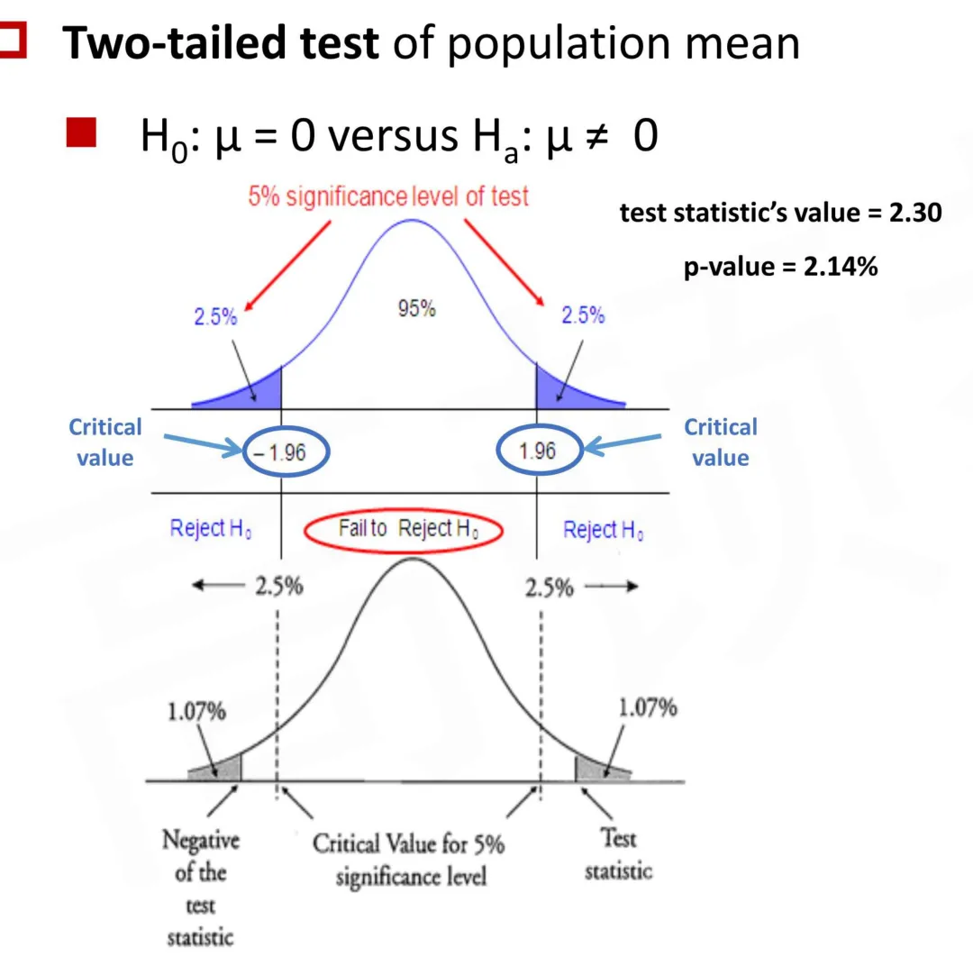
• Decision rule: If test statistic's value is outside the range of critical value (≥ upper critical value, or ≤ lower critical value), reject the null hypothesis; If the p-value is less or equal to the level of significance (α), reject the null hypothesis
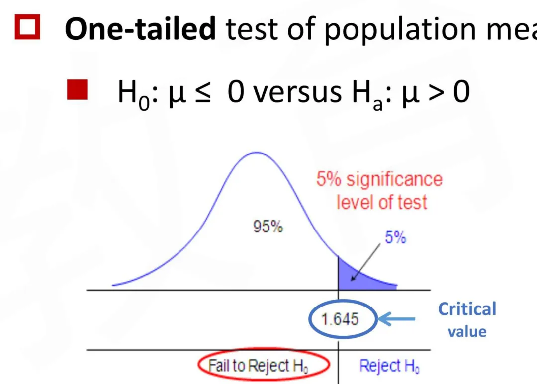
• Two-tailed test: H₀: μ = 0 vs Hₐ: μ ≠ 0; 5% significance → 2.5% in each tail; critical values −1.96 and +1.96. One-tailed test: H₀: μ ≤ 0 vs Hₐ: μ > 0; 5% in right tail; critical value 1.645
• Type I error is rejecting null hypothesis when it is true; P(Type I Error) = significance level α
• Type II error is failing to reject the null hypothesis when it is false; P(Type II Error) = β
• Power of test is rejecting the null hypothesis when it is false; Power of test = 1 − β
• Statistical significance does not necessarily imply economic significance, due to: Transactions costs; Taxes; Risk
• Test statistics: 单一正态均值(σ已知)z = (X̄−μ₀)/(σ/√n);σ未知 tₙ₋₁ = (X̄−μ₀)/(s/√n)。两独立总体均值差:方差相等假设下 t 检验 df = n₁+n₂−2;配对比较(相依总体)t 检验 df = n−1。单一方差 χ²ₙ₋₁ = (n−1)s²/σ₀²;两方差 F = S₁²/S₂²,df = (n₁−1, n₂−1);相关系数 tₙ₋₂ = r√(n−2)/√(1−r²)
• Example: Researcher believes a fund's mean returns (μ) exceed 1% per month. Sample size 36, sample mean 1.5%, sample standard deviation 1.8%, population normal. 1. H₀: μ ≤ 0.01 and Hₐ: μ > 0.01; 2. unknown variance, large sample → one-tailed z-test; 3. critical z at 5% = 1.65; 4. reject H₀ if z > 1.65; 5. Z = (0.015−0.01)/(0.018/√36) = 1.667 > 1.65; 6. Reject the null hypothesis
💡 学霸速记 假设检验外号“用数据打官司”,七步流程:设假设→选检验统计量→定显著性水平→定决策规则→收集数据算统计量→做统计决策→做经济决策。最后一步很妙:统计显著 ≠ 经济显著,因为还有交易成本、税、风险。两类错误外号“冤枉好人与放走坏人”:Type I 是原假设为真你却拒绝了(假阳性),概率 α;Type II 是原假设为假你却接受了(漏报),概率 β;检验功效 Power=1−β,是“有罪就该判”的能力。 |
⚠️ 避坑提醒 单尾还是双尾看 Hₐ 的符号:“≠”是双尾,把 5% 劈成两个 2.5%,临界值 ±1.96;“>”或“<”是单尾,5% 全给一边,临界值 1.645。用错尾巴,全盘皆输。 |
📝 习题演练 The probability of a Type II error for a hypothesis test is 15%. The power of the test is closest to: A. 85% B. 15% C. 5% ✅ 答案:A 📖 解析:Power of test = 1 − P(Type II Error) = 1 − β = 1 − 0.15 = 85%。功效是在原假设为假时正确拒绝它的概率;选项C(5%)是显著性水平的干扰项。 |
LOS 7.3 · compare and contrast parametric and non-parametric tests, describe situations in which each is the more appropriate type of test, construct appropriate hypothesis tests, and interpret the results
• Parametric tests are based on assumptions about population distributions and population parameters
• Nonparametric tests are applied when: Data do not meet distributional assumptions; Data are given in ranks; The hypothesis we are addressing does not concern a parameter
• If we want to test whether there is a relationship between the row and column, we can perform a test of independence using a non-parametric test statistic that is chi-square distributed
• χ² = Σ(Oᵢⱼ − Eᵢⱼ)² / Eᵢⱼ; The number of degrees of freedom is (r − 1)(c − 1)
💡 学霸速记 参数检验要假设总体分布和参数(比如正态);非参数检验在三种情况用:数据不满足分布假设、数据只有秩(ranks)、假设不涉及参数。 |
⚠️ 避坑提醒 列联表独立性检验用卡方:χ²=Σ(Oᵢⱼ−Eᵢⱼ)²/Eᵢⱼ,自由度 (r−1)(c−1)。看到 ranks / not normal / not about a parameter → 选非参数。 |
📝 习题演练 An analyst wants to test whether the rank ordering of fund managers' performance is random, using data expressed only as ranks. Which type of test is most appropriate? A. A parametric test based on the normal distribution B. A nonparametric test C. A z-test for the population mean ✅ 答案:B 📖 解析:数据以秩(ranks)形式给出、且检验假设不涉及总体参数,属于非参数检验的典型适用情形。参数检验(如z/t检验)要求总体分布与参数假设(如正态性)成立。 |
Topic 8 · The Return and Risk of a Financial Portfolio(投资组合的收益与风险)
LOS 8.1 · calculate, interpret, and evaluate the expected return, variance, standard deviation, covariance, and correlation of portfolio returns
组合收益与风险的计算:
• Expected return:E(R_p) = w₁E(R₁) + w₂E(R₂) + … + wₙE(Rₙ),即各资产期望收益的加权平均,权重为市值占比。
• Two-asset portfolio variance:σ_p² = w₁²σ₁² + w₂²σ₂² + 2w₁w₂Cov(R₁,R₂) = w₁²σ₁² + w₂²σ₂² + 2w₁w₂ρ₁₂σ₁σ₂;组合标准差 σ_p = √σ_p²。
• n资产组合方差:σ_p² = ΣᵢΣⱼ wᵢwⱼCov(Rᵢ,Rⱼ),协方差项(含自身方差)是组合风险的来源。
• 相关系数 ρ₁₂ = Cov(R₁,R₂)/(σ₁σ₂);ρ < 1 时分散化降低组合风险;ρ = −1 时存在可完全对冲风险的权重。
💡 学霸速记 组合收益是加权平均,但风险不是!这就是整个主题的灵魂。两资产组合方差外号“风险拼图”:σ_p² = w₁²σ₁² + w₂²σ₂² + 2w₁w₂ρσ₁σ₂。关键在相关系数 ρ:ρ=1 完全同涨同跌,分散化没用;ρ 越小组合风险越低;ρ=−1 还能找个权重把风险完全对冲掉——这就是“不要把所有鸡蛋放一个篮子”的数学证明。 |
⚠️ 避坑提醒 组合收益是加权平均,组合标准差不是!例:60% 投 A(σ=20%)、40% 投 B(σ=30%)、ρ=0.5,σ_p²=0.6²×0.2²+0.4²×0.3²+2×0.6×0.4×0.5×0.2×0.3=0.0432,σ_p≈20.8%。直接 60%×20%+40%×30%=24% 是错的,那是收益的算法,风险必须套方差公式再开根。 |
📝 习题演练 A portfolio is 60% invested in Asset A (standard deviation 20%) and 40% in Asset B (standard deviation 30%). The correlation between A and B is 0.50. The portfolio standard deviation is closest to: A. 20.8% B. 24.0% C. 25.0% ✅ 答案:A 📖 解析:σ_p² = 0.6²×0.20² + 0.4²×0.30² + 2×0.6×0.4×0.5×0.20×0.30 = 0.0144 + 0.0144 + 0.0144 = 0.0432;σ_p = √0.0432 ≈ 20.8%。选项B(24%)是把权重与标准差直接加权平均,忽略了方差-协方差结构。 |
LOS 8.2 · describe, calculate, and interpret the minimum-variance portfolio and portfolios that lie on the efficient frontier
最小方差组合与有效前沿:
• Minimum-variance frontier(最小方差前沿):在给定期望收益水平下,风险(方差/标准差)最小的所有组合构成的曲线。
• Global minimum-variance portfolio(全局最小方差组合):整条前沿上风险最低的组合,位于前沿最左端。
• Efficient frontier(有效前沿):最小方差前沿中位于全局最小方差组合之上的上半部分——在相同风险下期望收益最高、在相同收益下风险最低的组合集合;理性投资者只在有效前沿上选择组合。
• 分散化效果:资产间相关系数越低,前沿越向左(风险越低);ρ = 1 时前沿退化为直线。
💡 学霸速记 最小方差前沿和有效前沿就是“风险收益的菜单”:给定期望收益下风险最小的所有组合连成曲线叫最小方差前沿;上半段(全局最小方差组合往上)叫有效前沿——同样风险收益最高、同样收益风险最低,理性投资者只在前沿上选。全局最小方差组合就是整条曲线上风险最低的那个点。 |
⚠️ 避坑提醒 注意:最大化 Sharpe ratio 的不是全局最小方差组合,是切点组合(tangency portfolio)。资产间相关系数越低,前沿越靠左(风险越低);ρ=1 时前沿退化成直线。 |
📝 习题演练 Which statement about the global minimum-variance portfolio is most accurate? A. It has the lowest variance of any portfolio on the minimum-variance frontier B. It maximizes the Sharpe ratio among all risky portfolios C. It always contains equal weights of all assets ✅ 答案:A 📖 解析:全局最小方差组合是所有风险资产组合中方差最低的一个,位于最小方差前沿最左端。最大化Sharpe比的是切点组合(tangency portfolio),并非全局最小方差组合。 |
LOS 8.3 · explain the selection of an optimal portfolio, given an investor's risk aversion and the capital allocation line, and how this extends to the market portfolio and the capital market line
• Sharpe Ratio is a measure of excess return per unit of risk, thus the higher is better (only valid for positive Sharpe ratio)
• SRₚ = (Rₚ − r_b) / σₚ
• No units of measurement, so permits direct comparisons of dispersions across different data sets
资本配置线(CAL)与资本市场线(CML):
• Capital allocation line (CAL):由无风险资产与某一风险组合P构成的直线,E(R_c) = R_f + [(E(R_P) − R_f)/σ_P] × σ_c;其斜率即该风险组合的Sharpe比率。
• 最优组合选择:投资者按自身风险厌恶程度(效用函数)在CAL上选择无风险资产与风险组合的比例;风险厌恶越高,配置无风险资产越多。
• Market portfolio(市场组合):所有投资者都持有同一风险组合——由全部风险资产按市值加权构成,且该组合与无风险资产的连线(CML)相切于有效前沿。
• Capital market line (CML):以市场组合为风险组合的CAL,斜率 = (E(R_M) − R_f)/σ_M,即市场组合的Sharpe比率;CML上所有点都是无风险资产与市场组合的线性组合。
💡 学霸速记 夏普比率外号“性价比之王”:SR=(R_p−R_f)/σ_p,每单位总风险换多少超额收益,越高越好(只对正的 SR 有意义),无量纲可跨资产比。资本配置线 CAL 是无风险资产+某个风险组合的连线,斜率=该风险组合的 Sharpe 比率;投资者按风险厌恶程度在 CAL 上选位置,越怕风险越买无风险资产。 |
⚠️ 避坑提醒 市场组合是所有风险资产按市值加权的组合,它跟无风险资产的连线就是 CML——全市场唯一的“标准 CAL”。记死:CAL 的斜率就是所用风险组合的 Sharpe 比率;所有投资者风险厌恶不同,但他们面对的最优风险组合(市场组合)是同一个。 |
📝 习题演练 Which statement about the capital allocation line (CAL) is most accurate? A. The slope of a CAL equals the Sharpe ratio of the risky portfolio used B. All investors hold the same optimal risky portfolio regardless of risk aversion C. The CAL is the same line for every risky portfolio ✅ 答案:A 📖 解析:CAL的斜率 = (E(R_P) − R_f)/σ_P = 该风险组合的Sharpe比率。投资者因风险厌恶不同会选择CAL上的不同位置(选项B错误,那是假定了同一CAL上的最优比例对所有投资者相同);不同风险组合对应不同的CAL(选项C错误)。 |
Topic 9 · Simulation of Financial Asset Prices and Returns(金融资产价格与收益的模拟)
LOS 9.1 · describe historical simulation and explain how it can be used in investment applications
• Historical simulation uses randomly selected past data in risk factors to produce a distribution of possible outcome
• Limitations of historical simulation: Grounded in actual data and reflect only the risks represented in the sample historical data; Be limited used in scenario analysis
💡 学霸速记 历史模拟外号“翻旧账”:从过去真实数据里随机抽历史片段,生成未来可能结果的分布。局限:只反映样本历史里出现过的风险,没发生过的情景它看不见,所以情景分析里用处有限。 |
📝 习题演练 Which of the following is a limitation of historical simulation? A. It reflects only the risks that are present in the historical sample of data B. It requires assumed probability distributions for risk factors C. It cannot produce a distribution of possible outcomes ✅ 答案:A 📖 解析:历史模拟直接从过去数据中抽样,只能反映样本历史期内出现过的风险,无法刻画未发生过但可能发生的风险情景(因此也限制了它在情景分析中的用途)。假设分布是蒙特卡洛模拟的特征。 |
LOS 9.2 · describe bootstrap resampling, and explain how it can be used in investment applications
Bootstrap重抽样:
• Bootstrap resampling:从原始样本中有放回地反复抽取与原始样本等容量的许多“自助样本”,用这些样本统计量的分布来近似统计量的抽样分布。
• 用途:当解析公式不存在或分布假设难以满足时,用于估计统计量的标准误、构建置信区间、检验稳健性(如估计投资组合收益均值/标准差的标准误)。
• 与历史模拟的区别:Bootstrap针对“样本统计量的抽样分布”(估计量推断);历史模拟针对“未来结果的可能分布”(情景生成)。
💡 学霸速记 Bootstrap 外号“反复抽”:从原始样本有放回地反复抽等容量的自助样本,用它们的统计量分布近似抽样分布。用途:没有解析公式或分布假设难满足时,估标准误、建置信区间。核心特征:有放回! |
⚠️ 避坑提醒 看到 “with replacement from the original sample” → Bootstrap;看到 “assumed distributions” → Monte Carlo;看到 “only the risks in the historical sample” → Historical simulation。三个对应记牢直接送分。 |
📝 习题演练 In bootstrap resampling, each resampled dataset is drawn: A. with replacement from the original sample B. without replacement from the population C. from an assumed parametric distribution ✅ 答案:A 📖 解析:Bootstrap的核心特征是从原始样本有放回地抽样,从而近似统计量的抽样分布。选项C(假设参数分布)是蒙特卡洛的做法;无放回抽样则无法产生足够多的自助样本。 |
LOS 9.3 · describe Monte Carlo simulation and explain how it can be used in investment applications
• Monte Carlo simulation uses randomly generated values for risk factors, based on their assumed distributions, to produce a distribution of possible outcome
• Limitations of Monte Carlo simulation: Fairly complex; Do not directly provide precise insights; Provide answer no better than the assumption used
💡 学霸速记 蒙特卡洛外号“凭空造”:根据假定的风险因子分布随机生成海量情景,得到结果分布。局限:复杂、不给精确解析结论、结果“no better than the assumptions”——假设烂,输出烂。 |
📝 习题演练 Which statement about Monte Carlo simulation is most accurate? A. Its results are only as good as the assumptions made about the distributions of the risk factors B. It provides precise analytic insights into the pricing of derivatives C. It generates outcomes solely from historical data ✅ 答案:A 📖 解析:蒙特卡洛根据假定的风险因子分布随机生成大量情景,输出结果的质量受限于所用假设(“no better than the assumption used”);它不能提供精确的解析结论,也非基于历史数据抽样(那是历史模拟)。 |
Topic 10 · Applications of Simple Linear Regression in Finance(简单线性回归在金融中的应用)
LOS 10.1 · describe, interpret, and explain simple linear regression, including coefficient estimation using the least squares criterion
• The variable whose variation is being explained as the dependent variable, or the explained variable; The variable(s) whose variation is (are) being used to explain the variation of the dependent variable as the independent variable(s), or the explanatory variable(s)
• If we have only one independent variable, we refer to the method as simple linear regression (SLR)
• Yᵢ = b₀ + b₁Xᵢ + εᵢ, i=1,...,n — b₀ is the intercept; b₁ is the slope coefficient; εᵢ is the error term; E(ε) = 0
• Yᵢ = b̂₀ + b̂₁Xᵢ + eᵢ — b̂₀ and b̂₁ are the estimates of the population parameters; eᵢ = Yᵢ − Ŷᵢ
• In simple linear regression, the estimated intercept b̂₀, and slope b̂₁, are such that sum of the squared vertical distances from the observations to the fitted line is minimized
• SSE = Σ(Yᵢ − Ŷᵢ)² = Σ[Yᵢ − (b̂₀ + b̂₁Xᵢ)]² = Σeᵢ² (sum of squares error / residual sum of squares)
• The slope (b̂₁) is the ratio of the covariance between Y and X to the variance of X: b̂₁ = [Σ(Yᵢ−Ȳ)(Xᵢ−X̄)/(n−1)] / [Σ(Xᵢ−X̄)²/(n−1)] = Σ(Yᵢ−Ȳ)(Xᵢ−X̄) / Σ(Xᵢ−X̄)²
• Once estimate the slope (b̂₁), we can then estimate the intercept (b̂₀) using the mean of Y and the mean of X: b̂₀ = Ȳ − b̂₁ × X̄
💡 学霸速记 简单线性回归外号“画一条最合适的线”:用一个 X 解释一个 Y。Y 是被解释变量,X 是解释变量,只有一个 X 就叫简单线性回归。怎么画这条线?最小二乘法——让所有点到直线的垂直距离平方和最小。 |
⚠️ 避坑提醒 记两个公式:斜率 b̂₁=Cov(Y,X)/Var(X),截距 b̂₀=Ȳ−b̂₁X̄。回归线一定过均值点 (X̄,Ȳ),这是算截距的钥匙。例:Cov=48、Var=16、Ȳ=10、X̄=5 → b̂₁=3,b̂₀=10−3×5=−5。截距用减、别用加;斜率是 Cov/Var、别除反。 |
📝 习题演练 In a simple linear regression, the covariance between Y and X is 48, the variance of X is 16, the mean of Y is 10, and the mean of X is 5. The estimated slope and intercept are closest to: A. b̂₁ = 3.0 and b̂₀ = −5.0 B. b̂₁ = 0.33 and b̂₀ = 8.33 C. b̂₁ = 3.0 and b̂₀ = 25.0 ✅ 答案:A 📖 解析:b̂₁ = Cov(Y,X)/Var(X) = 48/16 = 3;b̂₀ = Ȳ − b̂₁X̄ = 10 − 3×5 = −5。选项B把斜率算成了Var/Cov的倒数;选项C在求截距时用了加法而非回归直线过均值点(X̄, Ȳ)的性质。 |
LOS 10.2 · describe and compare the assumptions of simple linear regression, identify violations through analyzing residuals, evaluate the estimated model's goodness-of-fit and regression coefficients, and results of ANOVA estimates
• 1. Assumption: the relationship between the dependent variable Y and the independent variable X is linear. When we look at the residuals of a model, what we would like to see is that the residuals are random, and the independent variable X is not random
• 2. Assumption: the variance of the regression residuals is the same for all observations, which is known as the homoskedasticity. If variance of residuals differs across observations, then we refer this as heteroskedasticity
• 3. Assumption: the observations, pairs of Yᵢ and Xᵢ, are independent of one another, which implies the regression residuals are uncorrelated across observations
• 4. Assumption: the regression residuals are normally distributed. This does not mean that the dependent and independent variables must be normally distributed
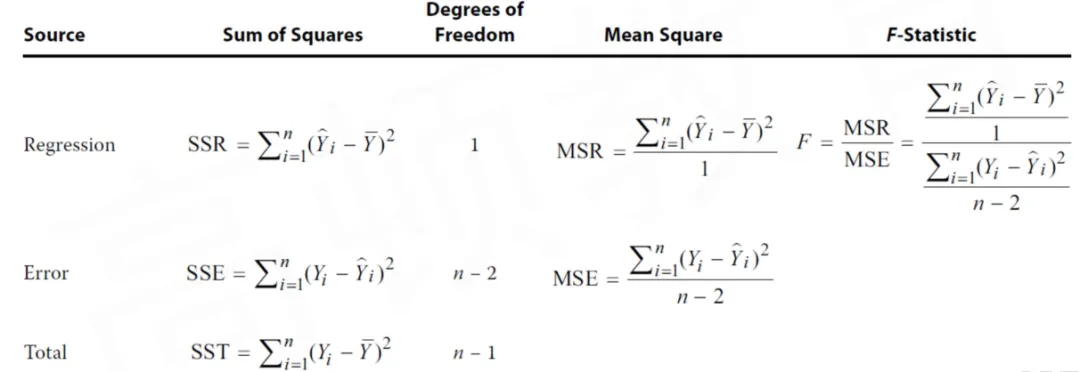
• ANOVA table: SSR = Σ(Ŷᵢ−Ȳ)² (df = 1, MSR = SSR/1); SSE = Σ(Yᵢ−Ŷᵢ)² (df = n−2, MSE = SSE/(n−2)); SST = Σ(Yᵢ−Ȳ)² (df = n−1); F = MSR/MSE
• Coefficient of determination (R²) = SSR/SST = 1 − SSE/SST; ranges from 0% to 100%; In a simple linear regression, R² = r² (square of the pairwise correlation)
• F = SSR/1 ÷ SSE/(n−2) = MSR/MSE, distributed with 1 and n − 2 degrees of freedom; H₀: b₁ = 0 vs Hₐ: b₁ ≠ 0
• sₑ = √MSE = √[Σ(Yᵢ−Ŷᵢ)²/(n−2)]; The smaller the sₑ, the better the fit of the model
公众号 财商的自我养成 里的一些有帮助的文章:
《【得分技巧】金融类考试逃不开的回归分析常见问题的解决》
《估计量好不好,全看这三个方面了》
⚠️ 避坑提醒 评价看 ANOVA 表和 R²:SST=SSR+SSE,R²=SSR/SST=1−SSE/SST,范围 0–100%,简单回归里 R²=相关系数的平方。F=MSR/MSE,检验 H₀:b₁=0。例:SST=200、SSR=150 → R²=150/200=0.75,X 解释了 Y 75% 的变异。sₑ=√MSE,越小拟合越好。 |
📝 习题演练 In a simple linear regression, SST = 200 and SSR = 150. The coefficient of determination is closest to: A. 0.75 B. 0.25 C. 0.50 ✅ 答案:A 📖 解析:R² = SSR/SST = 150/200 = 0.75,即自变量解释了因变量75%的总变异。选项B(0.25)误用了SSE/SST(=1−R²);选项C是把SSR当SST的一半。 |
LOS 10.3 · calculate and interpret predicted values, the standard error of the estimate, and prediction intervals for the dependent variable in a simple linear regression model and describe different functional forms
• Hypothesis tests of the slope coefficient: t = (b̂₁ − B₁)/s_b̂₁ ~ Tₙ₋₂; Feature of simple linear regression: t² = F; Hypothesis tests of the intercept: t ~ Tₙ₋₂
• Prediction interval of dependent variable: Ŷ_f ± t_critical(α/2) × S_f
• S_f = sₑ × √(1 + 1/n + (X_f − X̄)²/Σᵢ₌₁ⁿ(Xᵢ − X̄)²); The smaller standard error of the forecast (s_f) will be achieved, if X_f is close to X̄, n is large, and sₑ is small
• log-lin model: lnYᵢ = b₀ + b₁Xᵢ + εᵢ — The slope coefficient b₁ is the relative change in the dependent variable for an absolute change in the independent variable
• lin-log model: Yᵢ = b₀ + b₁lnXᵢ + εᵢ — The slope coefficient b₁ provides the absolute change in the dependent variable for a relative change in the independent variable
• log-log model: lnYᵢ = b₀ + b₁lnXᵢ + εᵢ — The slope coefficient b₁ is the relative change in the dependent variable for a relative change in the independent variable
💡 学霸速记 三种函数形式外号“换挡变速”:log-lin(lnY=b₀+b₁X)——X 绝对变动 1 单位,Y 相对变动 b₁;lin-log(Y=b₀+b₁lnX)——X 相对变动 1%,Y 绝对变动 b₁/100;log-log(lnY=b₀+b₁lnX)——X 相对变动 1%,Y 相对变动 b₁%,b₁ 就是弹性。 |
⚠️ 避坑提醒 log-log 的斜率是弹性——1% 对 1%,别把 0.80 当 80%!例:lnY=0.50+0.80lnX,X 涨 1% → Y 涨约 0.80%。log-lin 是绝对对相对、lin-log 是相对对绝对,别搞反。预测区间:X_f 离均值越近、样本越大、sₑ 越小,预测越准——别拿你的模型预测火星行情,越远离均值越没谱。 |
📝 习题演练 In the log-log regression model ln(Y) = 0.50 + 0.80 × ln(X), a 1% increase in X would most likely lead to: A. approximately a 0.80% increase in Y B. approximately a 1.25% increase in Y C. an 80% increase in Y ✅ 答案:A 📖 解析:log-log模型中斜率系数b₁是弹性:自变量相对变动1% → 因变量相对变动约0.80%。选项C混淆了“0.80”与“80%”;选项B是弹性的倒数,方向错误。 |
LOS 10.4 · calculate and interpret the variable estimates of the capital asset pricing model (CAPM)
CAPM的回归估计:
• CAPM:E(Rᵢ) = R_f + βᵢ[E(R_M) − R_f];其中βᵢ = Cov(Rᵢ, R_M)/Var(R_M),衡量资产对市场组合的系统性风险敏感度。
• 回归估计:用市场模型回归 Rᵢ − R_f = αᵢ + βᵢ(R_M − R_f) + εᵢ(或简式 Rᵢ = α + βR_M + ε),OLS估计出的斜率即β̂ᵢ,截距为α̂ᵢ(超额收益口径下,α代表非正常收益)。
• 解释:β > 1 为进攻型(放大市场波动)、β = 1 同步于市场、0 < β < 1 为防御型、β < 0 与市场反向。
💡 学霸速记 CAPM 回归估计:β=Cov(Rᵢ,R_M)/Var(R_M),衡量资产对市场组合的系统性风险敏感度。β>1 进攻型、β=1 同步、0<β<1 防御型、β<0 反向。用市场模型回归 Rᵢ−R_f=α+β(R_M−R_f)+ε,OLS 的斜率就是 β,截距 α 代表非正常收益。 |
⚠️ 避坑提醒 算期望收益先算市场风险溢价!例:R_f=2%、E(R_M)=10%、β=1.2 → E(R)=2%+1.2×(10%−2%)=2%+9.6%=11.6%。先算 (E(R_M)−R_f)=8% 再乘 β 再加 R_f,直接 1.2×10%+2% 是错误顺序。 |
📝 习题演练 The risk-free rate is 2%, the expected return on the market is 10%, and a stock's beta is 1.2. Using the CAPM, the required return on the stock is closest to: A. 11.6% B. 14.0% C. 12.0% ✅ 答案:A 📖 解析:E(Rᵢ) = R_f + β[E(R_M) − R_f] = 2% + 1.2×(10% − 2%) = 2% + 9.6% = 11.6%。选项B(14%)误用了1.2×10%+2%的错误乘加顺序;选项C(12%)漏掉了β对市场风险溢价的放大。 |
Topic 11 · Introduction to Financial Data Science(金融数据科学导论)
LOS 11.1 · describe how big data, machine learning, and artificial intelligence are used in financial data science, fintech, and investment management
• Numerical data (a.k.a. Quantitative data): continuous data & discrete data
• Categorical data (a.k.a. Qualitative data): nominal data & ordinal data
• Cross-sectional data; Time-series; Panel data
• Structured data; Unstructured data
大数据、机器学习与人工智能在金融中的应用:
• Big data(大数据):以3V为特征——Volume(体量大)、Velocity(产生/处理速度快,如高频交易tick数据)、Variety(种类多:结构化+非结构化,如新闻、社交媒体文本)。
• Machine learning(机器学习):监督学习(supervised:回归、分类,用于预测收益/违约概率)、非监督学习(unsupervised:聚类、主成分分析,用于客户分群、因子识别);自然语言处理(NLP)用于舆情与另类数据(alternative data)分析。
• AI / Fintech应用:智能投顾(robo-advisor)、算法交易、信用评分、欺诈检测、投资组合再平衡与风险管理。
💡 学霸速记 大数据三特征 3V 记死:Volume(体量大)、Velocity(速度快,如高频交易 tick 数据)、Variety(种类多,结构化+非结构化)。机器学习两大流派:监督学习有标签(回归预测收益、分类预测违约),非监督学习无标签(聚类做客户分群、主成分分析做因子识别)。NLP 处理舆情和另类数据;AI 应用:智能投顾、算法交易、信用评分、欺诈检测、组合再平衡、风险管理。 |
⚠️ 避坑提醒 高频交易数据毫秒级持续流动 → 对应 3V 里的 Velocity(速度)!体量大是 Volume,种类多是 Variety。看到这个对应,直接送分。 |
📝 习题演练 Which characteristic of big data is most directly associated with the continuous real-time flow of high-frequency trading data? A. Velocity B. Volume C. Variety ✅ 答案:A 📖 解析:Velocity指数据产生与处理的速度——高频交易数据以毫秒级持续流动,正是速度维度。Volume指数据规模之大,Variety指数据类型之多(结构化/非结构化)。 |

